
My dog rocks. Wilson is friendly to almost everyone (mailmen excepted) and he’s very soft. We’ve had him since he was a puppy and because the wife and I are dorky scientists, we’ve collected (non-invasive) data from him since day one. So today we’ll be modeling growth data, courtesy of Wilson, using R, the “nls” function, and the packages “car” and “ggplot2”. For reference, I drew on Fox and Weisburg (2010).

library("car"); library("ggplot2")
#Here's the data
mass<-c(6.25,10,20,23,26,27.6,29.8,31.6,37.2,41.2,48.7,54,54,63,66,72,72.2,
76,75) #Wilson's mass in pounds
days.since.birth<-c(31,62,93,99,107,113,121,127,148,161,180,214,221,307,
452,482,923, 955,1308) #days since Wilson's birth
data<-data.frame(mass,days.since.birth) #create the data frame
plot(mass~days.since.birth, data=data) #always look at your data first!
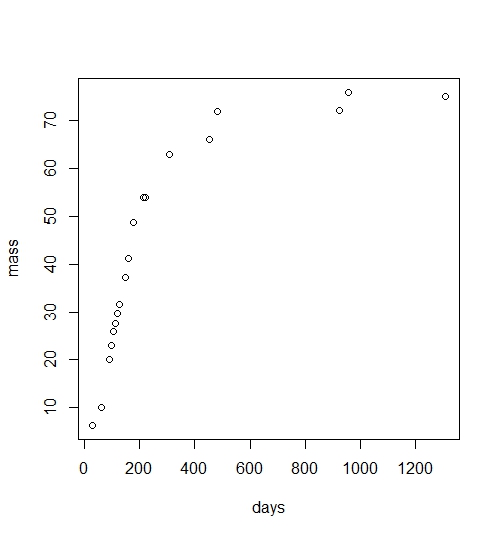
Wilson’s growth looks like a logistic function. As a puppy, he put on the pounds quickly (yep, I remember that), and he has flattened out around 75 lbs (thank god). Although I will say that he still thinks he is a lap dog.
A logistic growth model can be implemented in R using the nls function. “nls” stands for non-linear least squares.
The logistic growth function can be written as
y <-phi1/(1+exp(-(phi2+phi3*x)))
y = Wilson’s mass, or could be a population, or any response variable exhibiting logistic growth
phi1 = the first parameter and is the asymptote (e.g. Wilson’s stable adult mass)
phi2 = the second parameter and there’s not much else to say about it
phi3 = the third parameter and is also known as the growth parameter, describes how quickly y approaches the asymptote
x = the input variable, in our case, days since Wilson’s birth
One important difference between “nls” and other models (e.g. ordinary least squares) is that “nls” requires initial starting parameters. This is because R will iteratively evaluate and tweak model parameters to minimize model error (hence the least squares part), but R needs a place to start. There are functions in R that obviate the need for imputing the initial parameters, these are called “self starting” functions and in our case it would be the “SSlogis” function. But for now, we’ll skip that and give R some initial parameters manually.
coef(lm(logit(mass/100)~days.since.birth,data=data))
This calls for the coefficients of a linear model (slope and intercept) using the logit transform (log of the odds) and scaling the y by a reasonable first approximation of the asymptote (e.g. 100 lbs)
     (Intercept) days.since.birth
    -1.096091866      0.002362622
Then, we can plug these values into the nls function as starting parameters.
wilson<-nls(mass~phi1/(1+exp(-(phi2+phi3*days.since.birth))),
 start=list(phi1=100,phi2=-1.096,phi3=.002),data=data,trace=TRUE)
Here, we construct the model using the starting parameters. Trace returns the iterations.
3825.744 :  100.000  -1.096   0.002
3716.262 :  81.463877204 -0.886292540  0.002512256
3489.696 :  66.115027751 -0.731862991  0.003791928
1927.422 :  63.447368011 -1.036245947  0.007113719
204.0813 :  71.10755282 -2.06528377  0.01379199
123.3499 :  71.76966631 -2.39321544  0.01639836
121.3052 :  71.62701380 -2.45163194  0.01692932
121.2515 :  71.58084567 -2.46029145  0.01701556
121.2502 :  71.57256235 -2.46167633  0.01702943
121.2501 :  71.57121657 -2.46189524  0.01703163
121.2501 :  71.57100257 -2.46192995  0.01703198
121.2501 :  71.57096862 -2.46193546  0.01703204
The first column is the error (sums of squared error?) and the remaining columns are the model parameters. R took 11 iterations to reach model parameters it was happy with.
summary(wilson)
Formula: mass ~ phi1/(1 + exp(-(phi2 + phi3 * days.since.birth)))

Parameters:
      Estimate Std. Error t value Pr(>|t|)
phi1 71.570969   1.201983   59.54  < 2e-16 ***
phi2 -2.461935   0.162985  -15.11 6.88e-11 ***
phi3  0.017032   0.001227   13.88 2.42e-10 ***
---
Signif. codes:  0 ‘***’ 0.001 ‘**’ 0.01 ‘*’ 0.05 ‘.’ 0.1 ‘ ’ 1

Residual standard error: 2.753 on 16 degrees of freedom

Number of iterations to convergence: 11
Achieved convergence tolerance: 1.985e-06
We can see that our initial parameters weren’t too far off.
Next, let’s create the model predictions and plot the data. (I’ve noticed that copying and pasting this ggplot script isn’t working in R because of the quotation marks. Anybody know the solution for this? Temporarily, just substitute the quotation marks from this text with regular ones within R or R Studio.
#set parameters
phi1<-coef(wilson)[1]
phi2<-coef(wilson)[2]
phi3<-coef(wilson)[3]
x<-c(min(data$days.since.birth):max(data$days.since.birth)) #construct a range of x values bounded by the data
y<-phi1/(1+exp(-(phi2+phi3*x))) #predicted mass
predict<-data.frame(x,y) #create the prediction data frame#And add a nice plot (I cheated and added the awesome inset jpg in another program)
ggplot(data=data,aes(x=days.since.birth,y=mass))+
geom_point(color='blue',size=5)+theme_bw()+
labs(x='Days Since Birth',y='Mass (lbs)')+
scale_x_continuous(breaks=c(0,250,500,750, 1000,1250))+
scale_y_continuous(breaks=c(0,10,20,30,40,50,60,70,80))+
theme(axis.text=element_text(size=18),axis.title=element_text(size=24))+
geom_line(data=predict,aes(x=x,y=y), size=1)
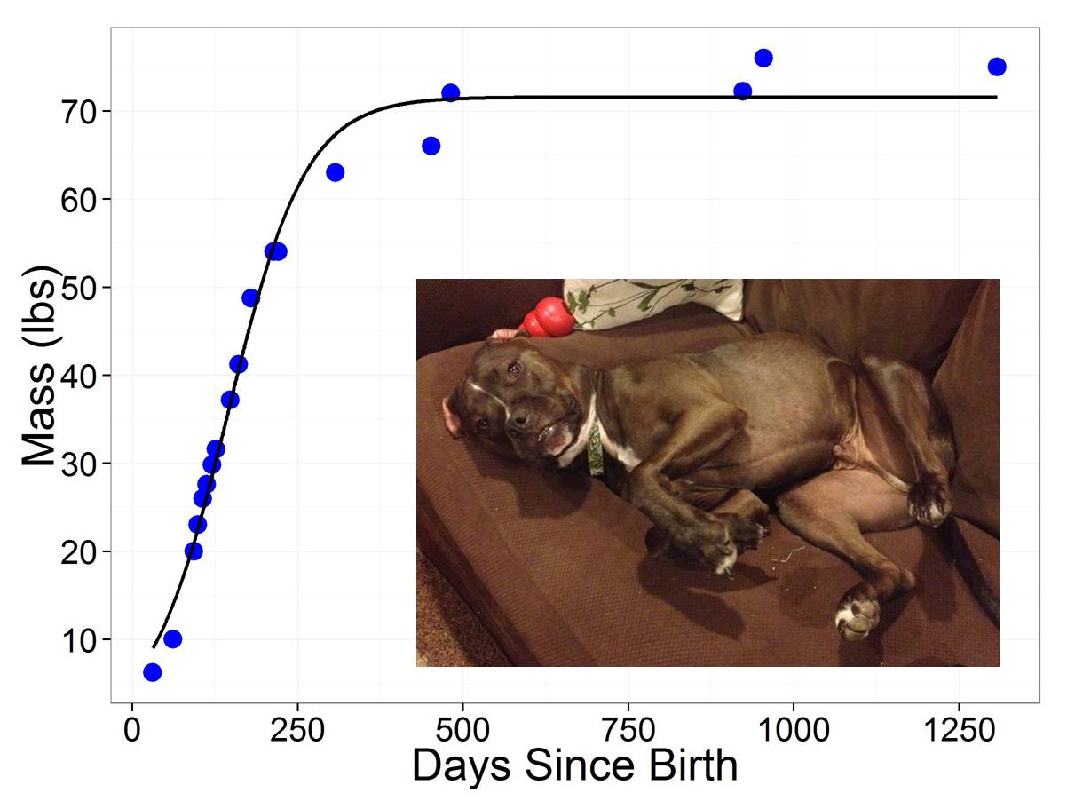
Hey, that looks like a pretty good model! It suggests that Wilson will asymptote at 71.57 lbs (Wilson, lose some weight buddy!). The model is under predicting his weight in the later region of the data, probably because of the two data points near the inflection point. Overall, I’m pretty happy with the model though!
There are some other packages (e.g. package “grofit” looks promising) and growth functions (e.g. gompertz) worth exploring because they can streamline some of the code, but we’ll save that for a future post.
Thanks for the data Wilson!
Check this out if you want to see how temperature affects whether Wilson is panting or not.

Thanks for nonlinear low down. What if I had multiple dogs in multiple groups? Could I use this package to tell me if my groups differed?
Hey Dustin! Yes you could totally use this to distinguish groups. I am unsure of the specific syntax using ‘nls’ but I’ve done similar things with logistic regression. Off the top of my head, you could look at parameter estimates between groups and see if they differed (e.g. compare confidence intervals of the estimates). If the groups had differing phi values that did not overlap, that would be evidence for different growth models. I will try and look at the code for this….
Looking at each parameter estimate independently would be a cool approach. I guess it would allow you to specify what aspect of growth differed among groups. Thanks.
This is GREAT, thank you so much
Thanks. What I will do if I have random growth rate. I mean if my gowth rates don’t have any trend or pattern over time like your example.
Growth rates typically follow some pattern, assuming resources are not limited. This is why most studies evaluate growth under ad libitum resource availability. I would first ask why your data don’t have any discernible trend. Second, what is your question of interest?
Dear Brian,
I am trying to fit the predicted curve on my data, but I think there is something wrong in the curve.
Can you review my script to look what is wrong?
Thank you very much for your attention.
Sincerely, Bruna
Hi Bruna, Send me your script and I’ll take a look! You can find my email on my “about” page.
Cheers,
Brian
Hi Brian, this was so helpful, thanks! Any way you could add in confidence intervals on either side of the predicted curve?
Hi Taryn! For an approximate 95 CI you could double the standard errors around the slope coefficients. But I think there is a better method involving pulling estimates from the profiled log-likelihood, which will allow for asymmetric CIs (I’ll have to look into this). Another approach would be to bootstrap the data and generate CIs that way. So for example, simulate 999 more Wilsons (with replacement) and calculate model coefficients. Then take the 2.5 and 97.5 percentiles of those models and there is your 95% CI.
Fantastic! Thanks.
Hi Brian,
I am very interested in this code! I am trying to predict the size of a given population using the following line of code:
predict.pop <- predict(pop, data.frame(time = c(2020, 2030)))
It works very well but I wonder if it would be possible to provide some confidence intervals along with these estimates as you discuss above with Taryn?
many thanks in advance!
a
Hi Antoine!
“confint(model)” will return the lower and upper 95% CI of the parameter estimates for your model. Try modeling both upper and lower bounds and using geom_ribbon to fill in the prediction. If this doesn’t make sense, perhaps I can generate a follow up post to highlight this. Cheers, Brian
thanks for being so responsive!
Your answer makes sense but I am struggling a little bit with my code.
By running the predict cmd, I get the expected pop size at a given year.
The LGM I used is the following:
nls(value ~ SSlogis(time, phi1, phi2, phi3), mydata)
it is based on the following webpage:
When I run confint on the model itself:
confint(nls(value ~ SSlogis(time, phi1, phi2, phi3),data=mydata)), it works but gives me the CI of phi1, phi2 and phi3.
My goal is to obtain the confint of predict…
I tried to adapt the model above with the given upper CI of phi1, phi2 and phi3 but was not successful
Thoughts?
I am happy to try an optimized/alternative model if you favor another one.
Here’s an example for a limited subpopulation (value=nb of subjects):
time value
2010 1
2011 1
2012 4
2013 6
2014 7
2015 8
2016 13
I’d like to predict the expected size in 2020, 2030 and CI…
thanks again!
a
Hi Brian,
I am reaching out to you again regarding the lgm model I am using. Thanks to your advices, I was able to run my model and got CI for phi1, phi2 and phi3 with the following:
model <- nls(size ~ SSlogis(date2, phi1, phi2, phi3), data = mydata)
confint(model)
The code above gives me the CI of all phis.
Next, I tried to estimate the predicted pop size in the future by doing this:
predict.model <- predict(model, data.frame(year = c(2020,2030,2040)))
…but I am still unable to generate the CI for the 'predicted pop size'. Any chance you can help me with that? Does that make sense?
thanks!
a
Hi Antoine!
Makes sense to me. I’m unsure if the predict function works for nls. Have you tried it the “long” way as in my post?
I’m traveling now but can look at this in earnest when I return in two days.
Cheers!
Thanks Brian!
predict function does work but no CI… I will try the ‘long’ way you suggest but if there is a more straightforward way, I am eager to learn how to do it!
Have a safe trip
a
Oops sorry. Misread your comment.
I’m not sure if plotting confidence intervals the long route is statistically sound. I’ll have to gander at the texts. Another solution would be to bootstrap simulate the data and plot the upper and lower bounds of the simulated data. We did this in a paper, let me know if you want to see that solution.
>
the bootstrap option seems promising. Can you redirect me to your paper? Do you have a code I could use attached to your publication? thanks again.
The paper is Komoroske et al 2014 Conservation Physiology (full citation on my publication page). But no code attached to the paper. I can share the code when I return to the states. Feel free to email me if you haven’t heard from me in a day or two!
>
thanks Brian,
I will email you in a couple of days. By then, I will read your paper.
Have a safe trip!
Hi Brian
Just a quick reminder. Any chance you can help me for getting CI (or bootstrap sim) for my dataset?
thanks again
Hello I am Victor, from Chile, I am glad to meet you and thank you for the explanation. Using your code for learning, I identify a little typing mistake, that blows some minutes my mind, in the 14th line phi1 does not have added the letter “-“, for the rest. I am grateful for you, because despite that spanish is my mother tongue, the spanish explanations were not clear for me. Best Regards from Southern Chile.
Thanks Victor! I’ve corrected the typo.
Thx Brian. Came to your blog after a long search for such an example on the implementation of a logistic growth model. Ggplot script worked immediately after pasting it to RStudio (mac OS) by the way.
Very nice explanation : )
Thank you!
Jorge
Awesome post, thanks!