There’s a lot of freely available data out there. Much of this data is spatial and derived from remote sensing platforms (e.g. satellites). Here’s a quick primer on using the package “raster” to plot and extract spatial data using the Bio-ORACLE dataset. The raster package was created by Robert Hijmans (go Aggies!) and there is a nice introduction available. If you’re not an SDMer (species distribution modeler) you might not know that Bio-ORACLE is a nifty dataset of 23 variables (temperature, chlorophyll, cloud fraction, etc.) available at 5 arcmin (9.2 km) resolution. Do check out the original paper describing this data! The files are compressed and available as “.rar” files, which you’ll need to decompress using something such as 7-Zip.

library (raster)
sst.mean<-raster("sstmean.asc")
sst.mean

Load the package and then create the raster file using the decompressed “.asc” file downloaded from Bio-ORACLE. Calling the object reveals the critical features (dimensions, extent, resolution). Thusly…..
class             : RasterLayer
dimensions : 1680, 4320, 7257600  (nrow, ncol, ncell)
resolution    : 0.08333333, 0.08333333  (x, y)
extent           : -180, 180, -70, 69.99999  (xmin, xmax, ymin, ymax)
coord. ref.    : NA data
source           : ~sstmean.asc
names           : sstmean

Now let’s plot something! In this case, sea surface temperature (SST), which comes from NASA’s MODIS instrument onboard the Aqua satellite. MODIS is a spectroradiometer. Lovely!

plot(sst.mean, main="SST") #plot raster

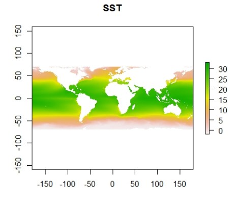
Those are some ugly colors so let’s tweak that and add a legend for the color bar at right.

 
plot(sst.mean,main="SST", col=colorRampPalette(c("blue","purple", "yellow","red"))(255),      legend.args=list(text='Degrees C', side=4,font=2, line=2.5, cex=0.8)) 

Let’s say we wanted to zoom in on a specific area. We could limit the X and Y coordinates of the plot.

 
 plot(sst.mean,main="Galapagos Islands", col=colorRampPalette(c("blue","purple", "yellow","red"))(255), 
legend.args=list(text='Degrees C', side=4,font=2, line=2.5, cex=0.8), xlim=c(-95,-95),ylim=c(-5,5)) 

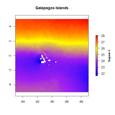
We could also overlay points and text on the map.

 
plot(sst.mean,main="Galapagos Islands", col=colorRampPalette(c("blue","purple", "yellow","red"))(255), 
legend.args=list(text='Degrees C', side=4,font=2, line=2.5, cex=0.8), xlim=c(-95,-95),ylim=c(-5,5))
points(cbind(-90,0), pch=21, cex=1, bg="red") 
text(x=-88.5,y=0, labels="Shark Bait") 

If I wanted the SST of the Shark Bait site above, I could extract the values from the raster.

 
extract(x=sst.mean,y=cbind(-90,0), method="simple") 

Shark Bait is a balmy 23.966 degrees C. The “simple” method extracts the value from that cell. We could also interpolate from the nearest 4 adjacent cells.

 
extract(x=sst.mean,y=cbind(-90,0), method="bilinear") 

Using the ‘bilinear interpolation’, we get 23.9265 degrees C. This interpolation can be handy if your specific cell lacks data, which can occur if cells are near the coast.

You could also easily scale up the overlaying of many points onto the raster, in addition to extraction of values.
Finally, since the raster dataset is just a bunch of numbers, we can make univariate plots as well.

hist(sst.mean, main="Mean SST Frequency Distribution", xlab="Temperature C", maxpixels=ncell(sst.mean)) #histogram of SSTs

Whoa, the oceans have a weird bimodal SST signature going on. Someone should look into that….

Happy rastering!

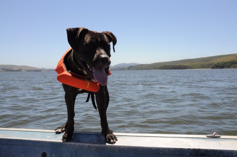
Obligatory Wilson pic (on a boat!) in…

3…

2…

1…